FIR model
Overview
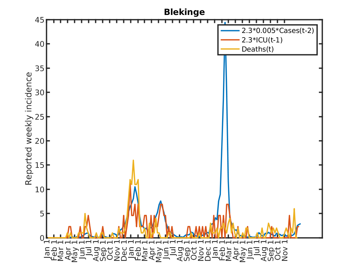
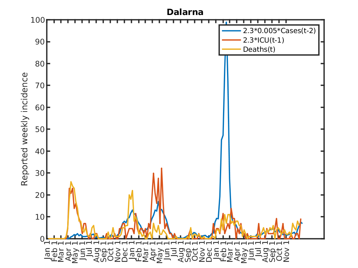
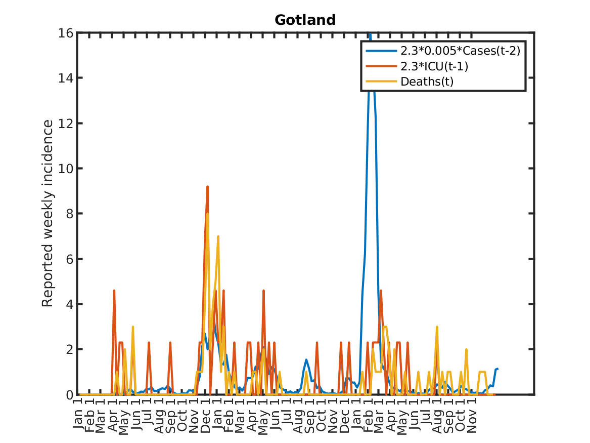
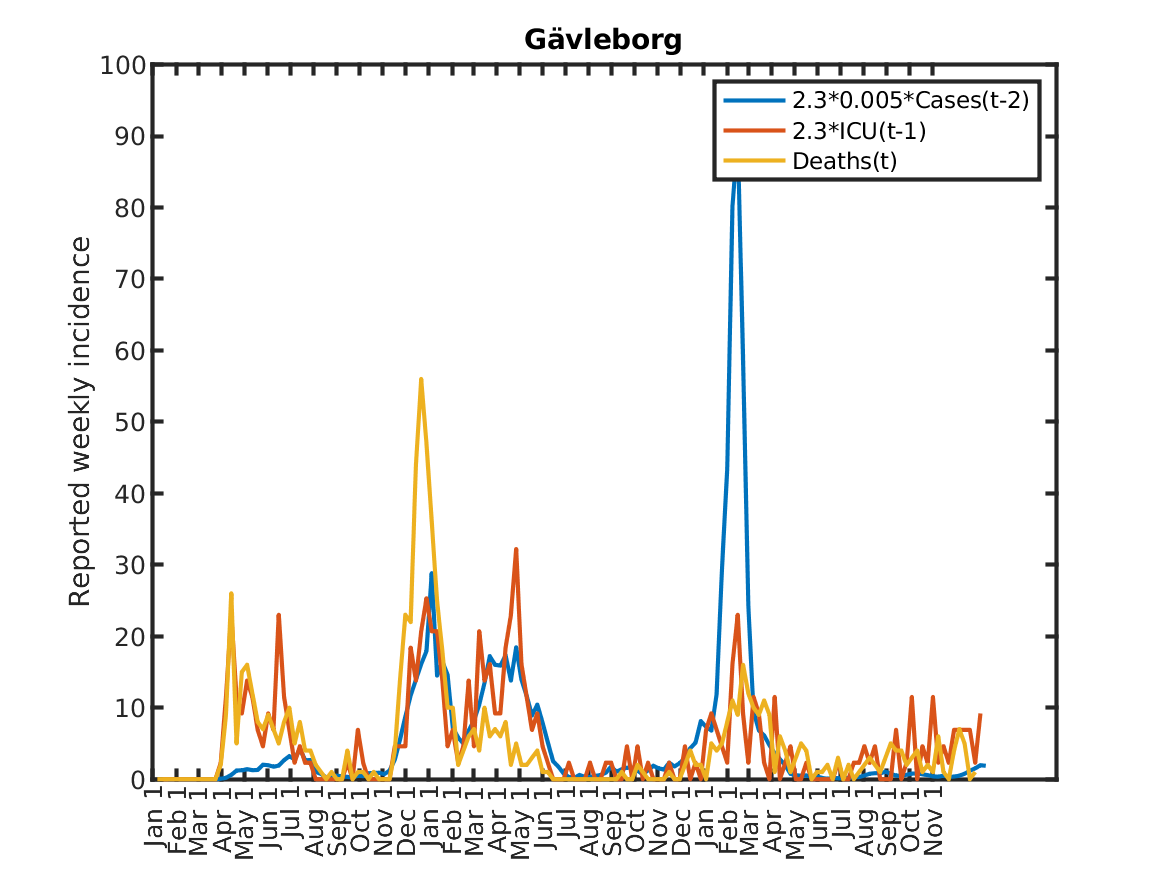
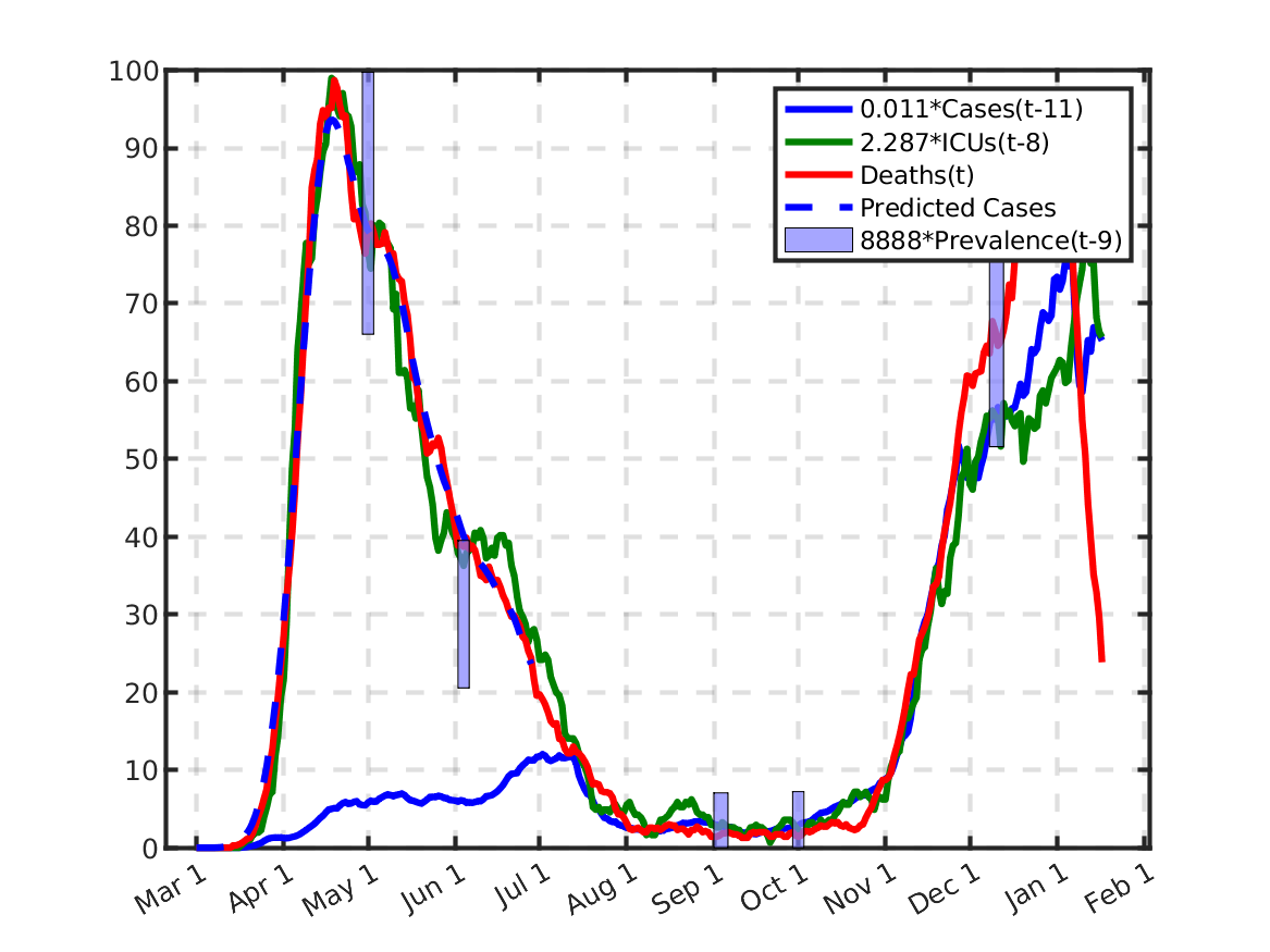
Data from The Swedish Public Health Agency shows a strong correlation between reported daily ICU admittance (ICU) and the reported number of new daily deaths (deaths). Further, there is an almost as strong correlation between ICU and the number of daily new PCR-confirmed cases (Cases) since July 2020, by when testing capacity had increased to facilitate free-of-charge self-tests to all symptomatic citizens (and strong encouragement for symptomatic individuals to self-test was communicated by the Swedish government).
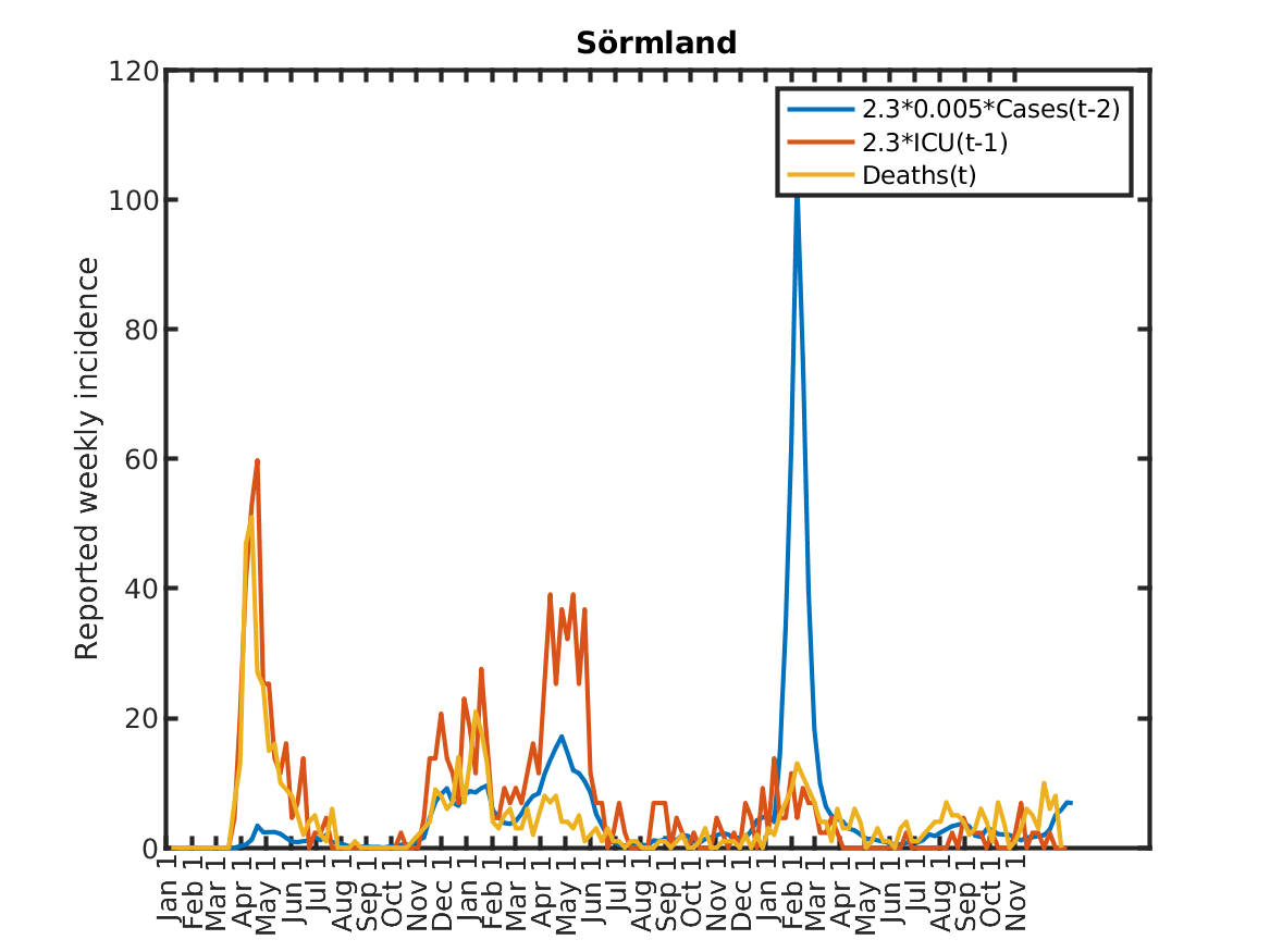
The following plot shows the relations, originally discovered by Prof. Andreas Wacker at Lund University. He found that if you multiply the number of ICU patients by 2.3, you can fairly accurately predict the number of deaths the following week. Further, the number of newly admitted ICU patients the next week can be predicted by dividing the number of new cases during the current week by 200. As a consequence, the number of new deaths over one week in two weeks time is approximately 2.3/200 times the number of new cases this week. This shows that a very simple model of the IFR (infection to fatality ratio) and the delay between infection and death is sufficient to explain historic data in Sweden.
Estimating the delay and gain
The abbreviation FIR means finite impulse response and is used in control theory to fit a running average of an input variable to an output variable. A pure gain and delay is a special case of an FIR model.
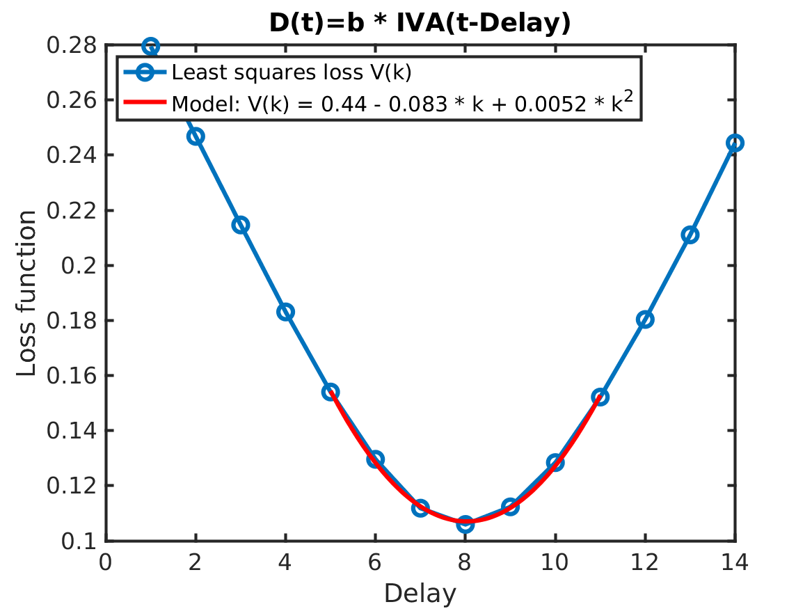
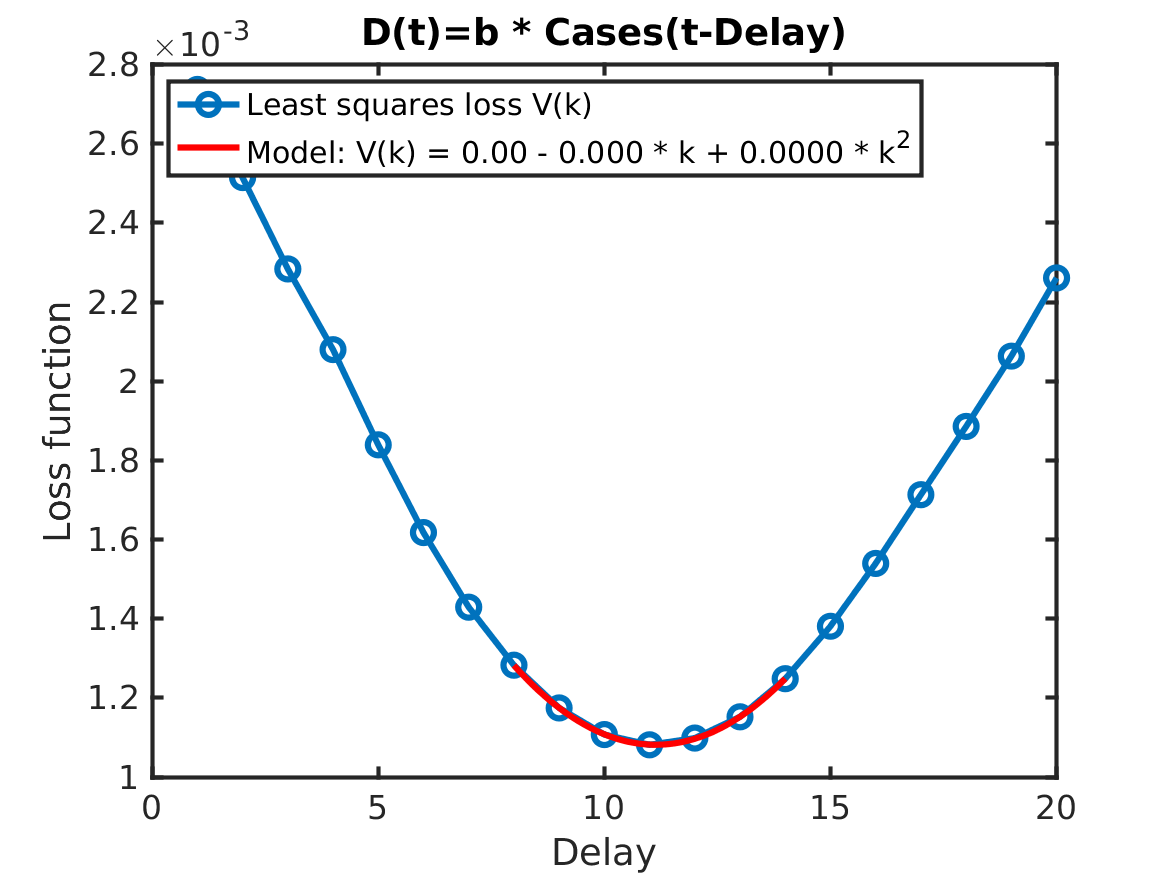
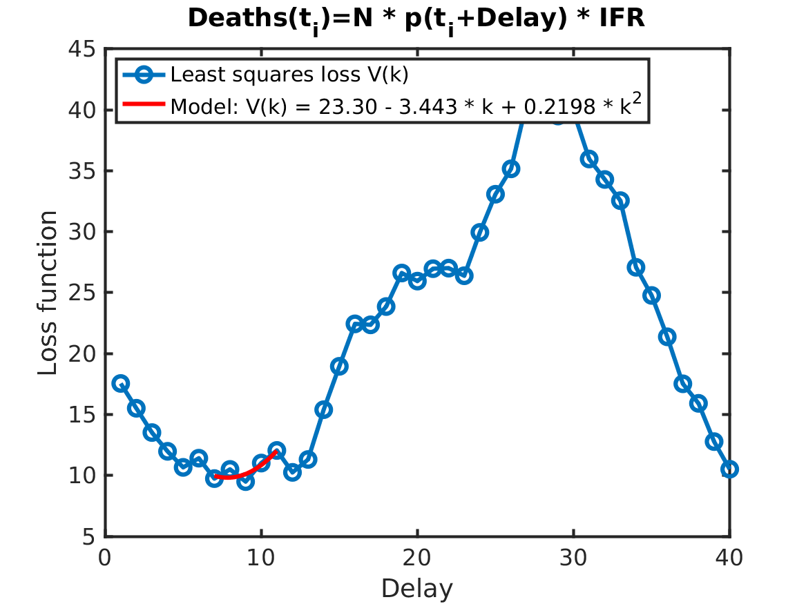
To improve the delay estimate (one week between cases and ICU; one week between ICU and death) and the gain estimate (a factor 1/2.3 between ICU and death; a factor 1/200 between cases and ICU), we can solve a simple regression problem. For the gain, the ordinary least squares method is used. For the delay, an exhaustive search is used. For each delay candidate the best gain is found, and then the delay-gain pair that best explains the data is chosen. The quadratic loss function V(delay), plotted below, is used to judge how well a particular delay-gain pair explains the data. We can see that close to its minimum the loss function can be well approximated by quadratic function, plotted in red. The coefficient of the quadratic term in this function defines its curvature and can be interpreted as the variance of the delay estimate. It tells us how sensitive the model is to small variations of the estimated delays. In the studied case, the curvature of the red curve corresponds to a 0.1 day standard deviation in the delay estimate. This tells us that the best fit of the delay between positive PCR tests (cases) and ICU admittances is 9 days plus minus a couple of hours, thus quite a clear correlation. Further, the standard deviation printed in the title shows the average size of the error in using PCR tests as a proxy for ICU admittances, which again indicates a very clear correlation.
This estimation methodology makes it possible to estimate a fractional delay and its standard deviation. The result is summarised in the table below.

Estimating IFR from prevalence tests
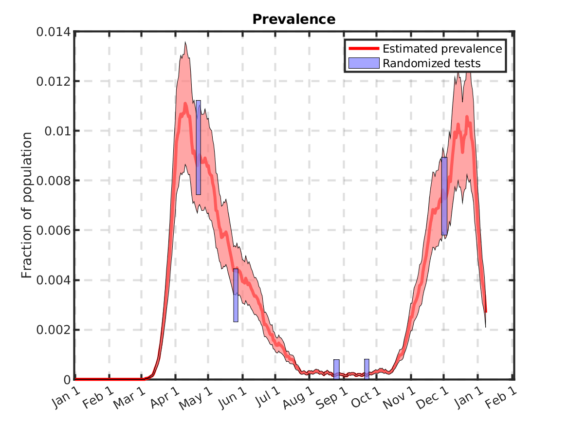
Prevalence tests have been performed on five occasions as summarised in the table below.
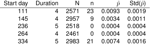
We can use this data together with reported mortality data to estimate the infection to fatality ratio (IFR). First, the proportion of the population infected at the time period of the test is computed as n/N. We use the rather non-informative prior Beta(1,1)=U(1,1), which avoids the problem of estimating standard deviation zero in cases when no positive cases where found. In a second step, a linear regression problem is solved to estimate IFR from the five prevalence tests compared to the mortality rate a number of days later. Also this delay is estimated using LS.
The estimated parameters are summarised below.
![]()
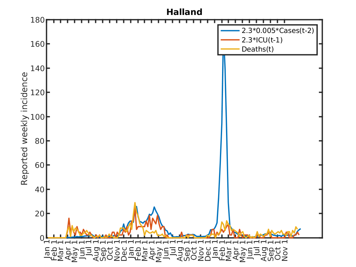
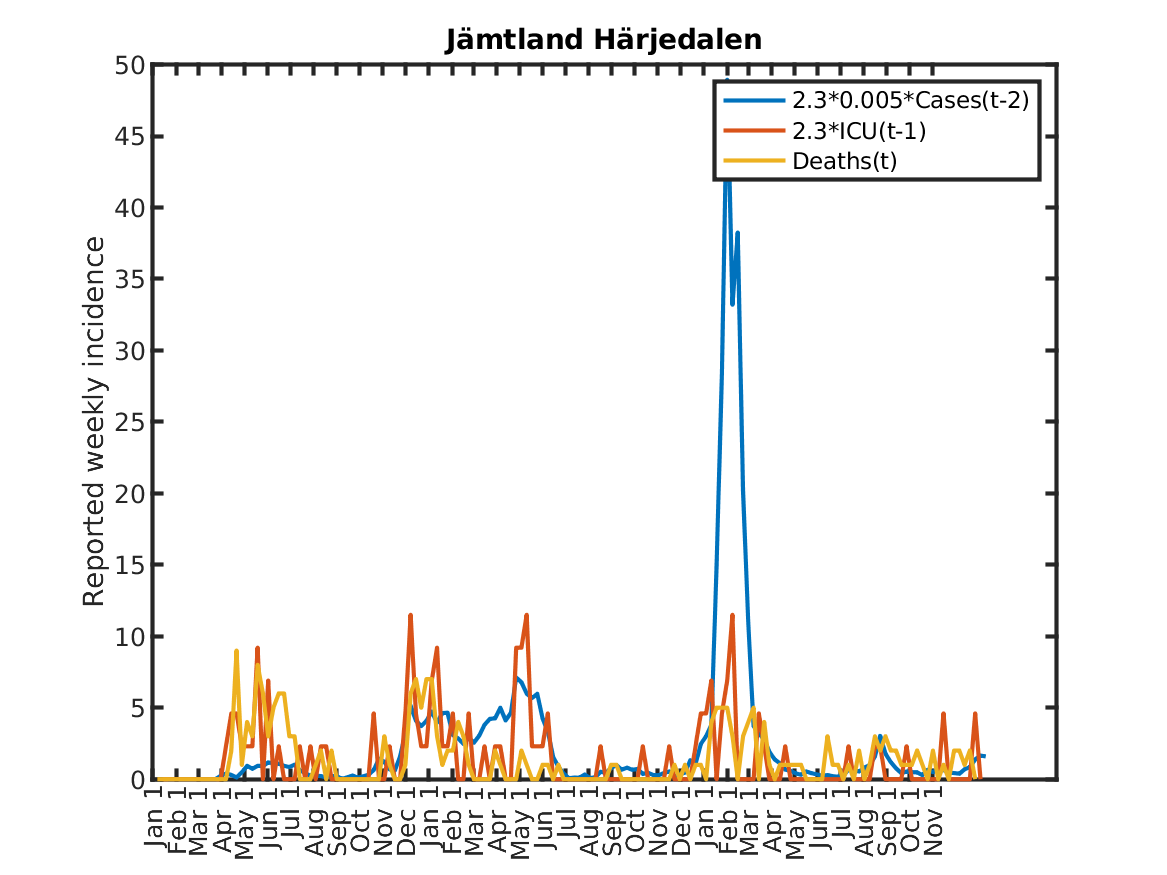
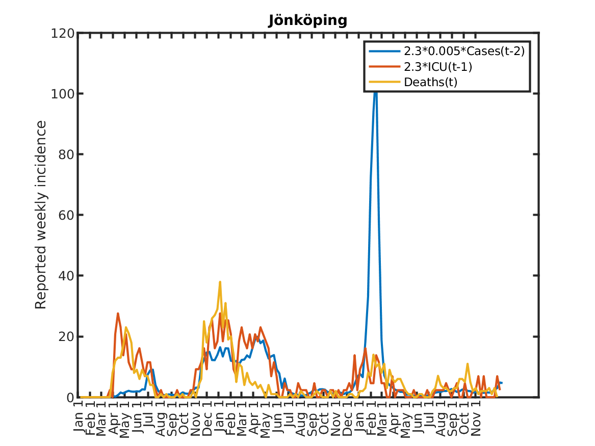
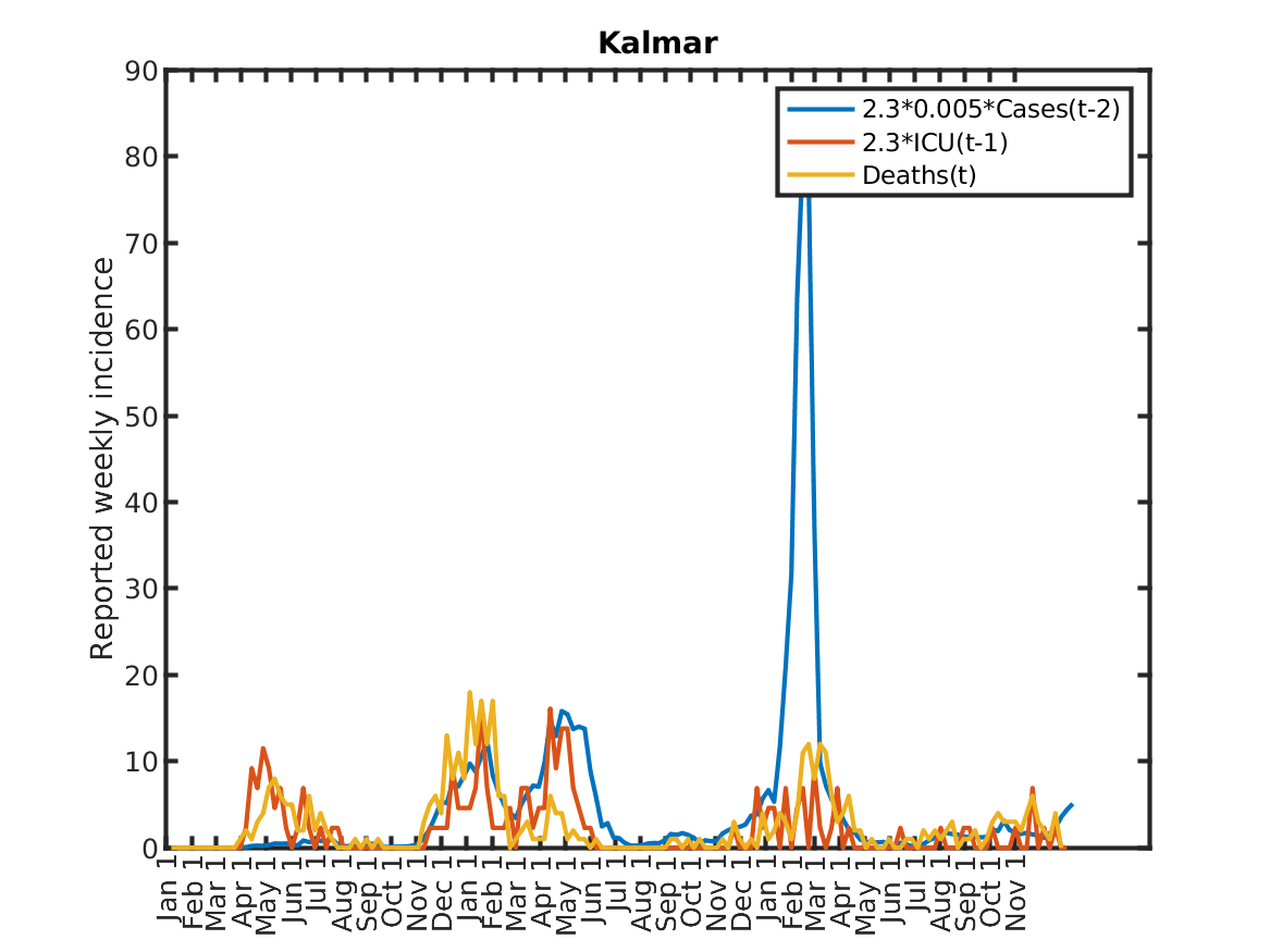
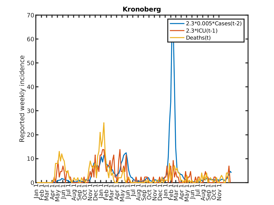
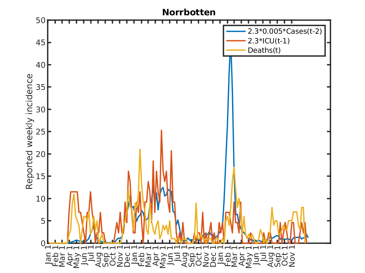
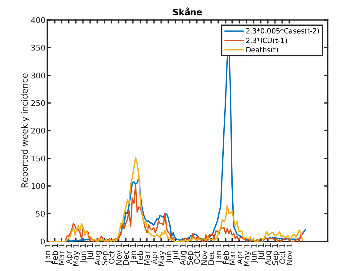
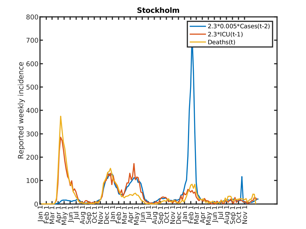
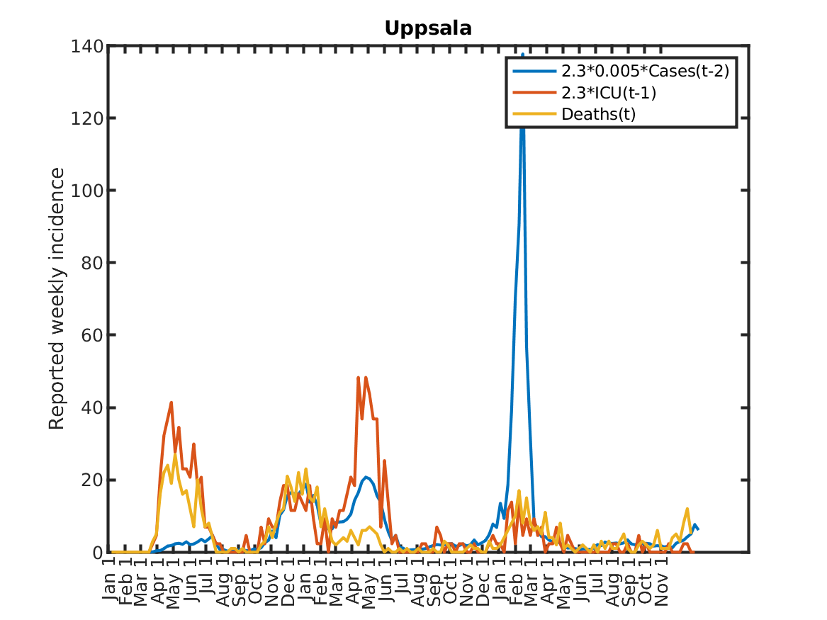
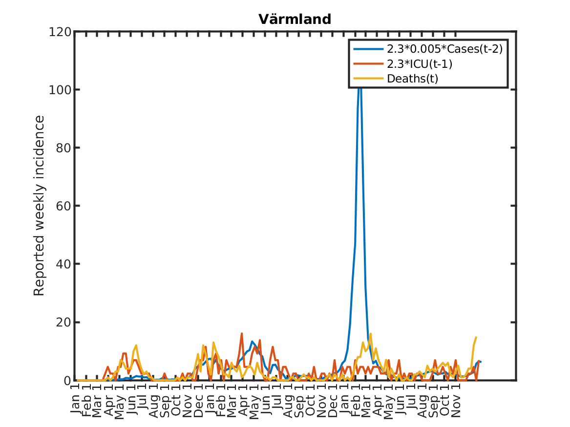
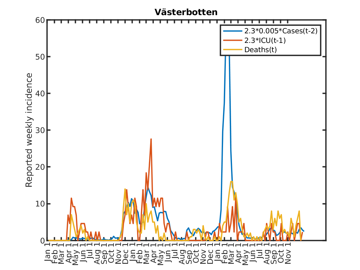
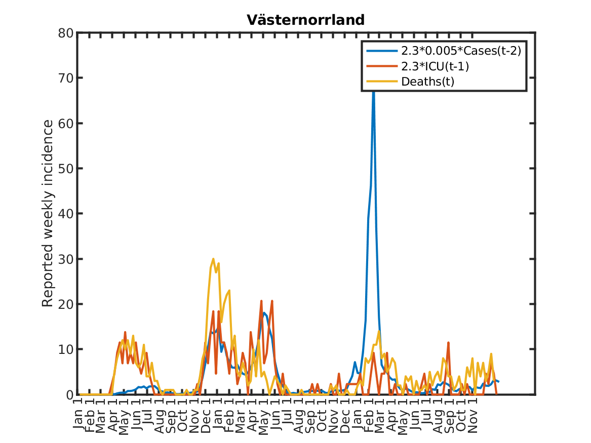
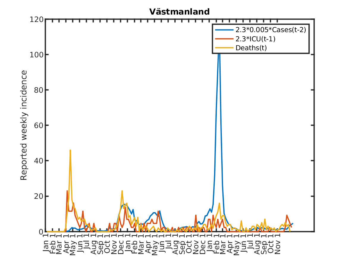
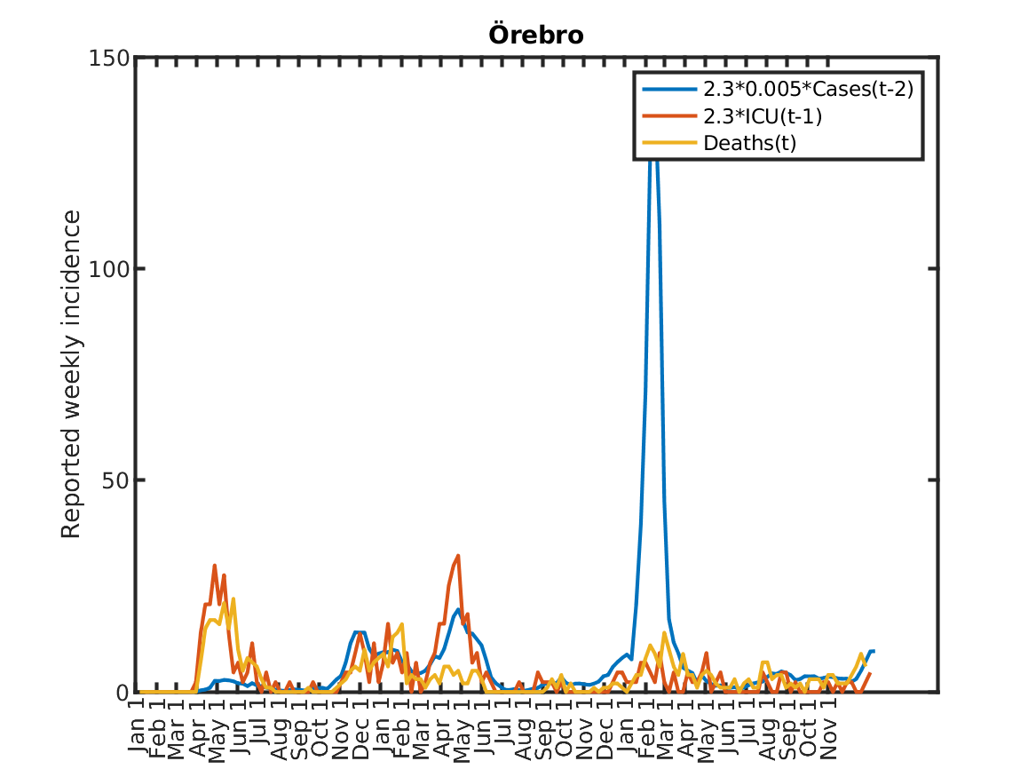
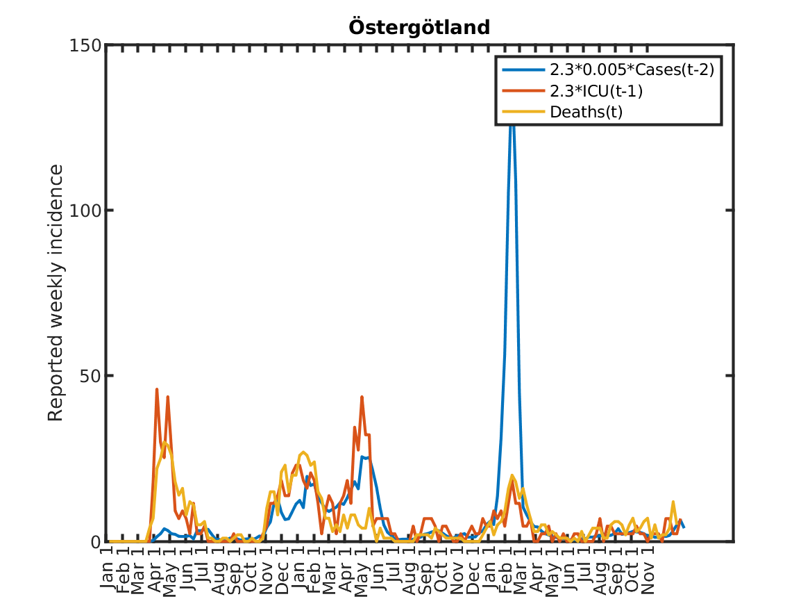
Results for individual regions
Plots in alphabetic order for each region in Sweden.